


How to Measure Magnetic Field Strength and Verify Shield Performance
Posted by Josh Wickler, Vice President of R&D on Nov 14th, 2026
Key Takeaways
- Select the Right Instrument:* Use a fluxgate magnetometer for low-field measurements (< 100 µT) inside shields and a Hall effect probe for high-field source characterization (> 1 mT).
- Establish a Baseline:* Before installing a shield, measure the ambient DC and AC magnetic field at the location over a full operational cycle to establish an accurate denominator for your shielding factor calculation.
- Follow a Disciplined Protocol:* Measure the residual field at the geometric center of the enclosure, recording all three vector components (Bx, By, Bz) to calculate the total field magnitude.
- Measure Before and After Annealing:* Fabrication stress severely degrades permeability. Measuring a shield before and after final hydrogen annealing is the only way to quantify the permeability recovery and validate final performance.
- Measure Across Frequencies:* A single DC reading is insufficient. Characterize shield performance at the specific frequencies of your interference sources (e.g., 60 Hz) as DC and AC attenuation mechanisms differ.
An engineering team installs a new MuMETAL® enclosure around a sensitive magnetometer array. They take a single DC gaussmeter reading at the geometric center, see a number below their target, and declare the shield validated. Six weeks later, the instrument exhibits intermittent noise that traces back to 60 Hz AC interference the DC reading never captured. The qualification data is now suspect, and the project is at risk.
This scenario is common. Successful magnetic shielding depends on verifiable performance, and verifiable performance depends on disciplined measurement. The instrument you choose, where you place the probe, how you characterize the ambient baseline, and whether you measure across the relevant frequency spectrum determine whether your shielding data is a meaningful engineering asset or a source of false confidence.
This guide is written for engineers, program managers, and laboratory leaders tasked with validating shield performance in demanding electronics, aerospace, medical, and scientific research applications. It provides a practical framework for how to measure magnetic field strength in a way that produces trustworthy, defensible data. We will cover:
- Units and reporting conventions for shielding specifications
- Instrument selection for low-field measurement
- Ambient baseline characterization
- In-shield measurement protocol
- Frequency-dependent considerations
- Post-annealing performance verification
- Correlating simulation with physical measurement
The goal is not just to take a reading, but to implement a protocol that confirms your shield delivers the required attenuation under real operating conditions.
Units and Reporting Conventions for Shielding Specifications
Inconsistent unit usage between measurement reports, simulation outputs, and supplier datasheets is a frequent source of miscommunication that stalls procurement and design reviews. Establishing a clear convention is the first step in any measurement plan.
The primary SI unit for magnetic flux density (B) is the tesla (T). However, the CGS unit, the gauss (G), remains widely used in North American shielding work. The conversion is straightforward:
1 T = 10,000 G
For the extremely low frequency magnetic fields relevant to shielding validation, these units are too large to be practical. The working units are typically nanotesla (nT) and milligauss (mG).
- 1 µT = 1,000 nT
- 1 G = 1,000 mG
- 1 µT = 10 mG (or 1 nT = 0.01 mG)
To put this in context, Earth's magnetic field at mid-latitudes is approximately 25,000 to 65,000 nT (250 to 650 mG). This ambient field is the baseline that most shields are designed to attenuate. A specification requiring a residual field of 50 nT (0.5 mG) is asking for a shielding factor of roughly 1,000 against the geomagnetic field.
It is also important to distinguish magnetic flux density (B) from magnetic field intensity (H), which is measured in amperes per meter (A/m). While related through the material's permeability, they are not interchangeable. A specification that states "40 dB attenuation" without specifying the frequency, field orientation, ambient reference value, and unit of measurement is incomplete and can lead to procurement disputes.
Practical Recommendation: When reporting any shielding measurement, always state the unit (e.g., nT or mG), the measurement axis or total vector magnitude, the sensor type used, and the ambient reference field against which the shielding factor was calculated. For more background on shielding terminology and principles, visit our shielding FAQs.
Choosing the Right Instrument for Low-Field Magnetic Measurement
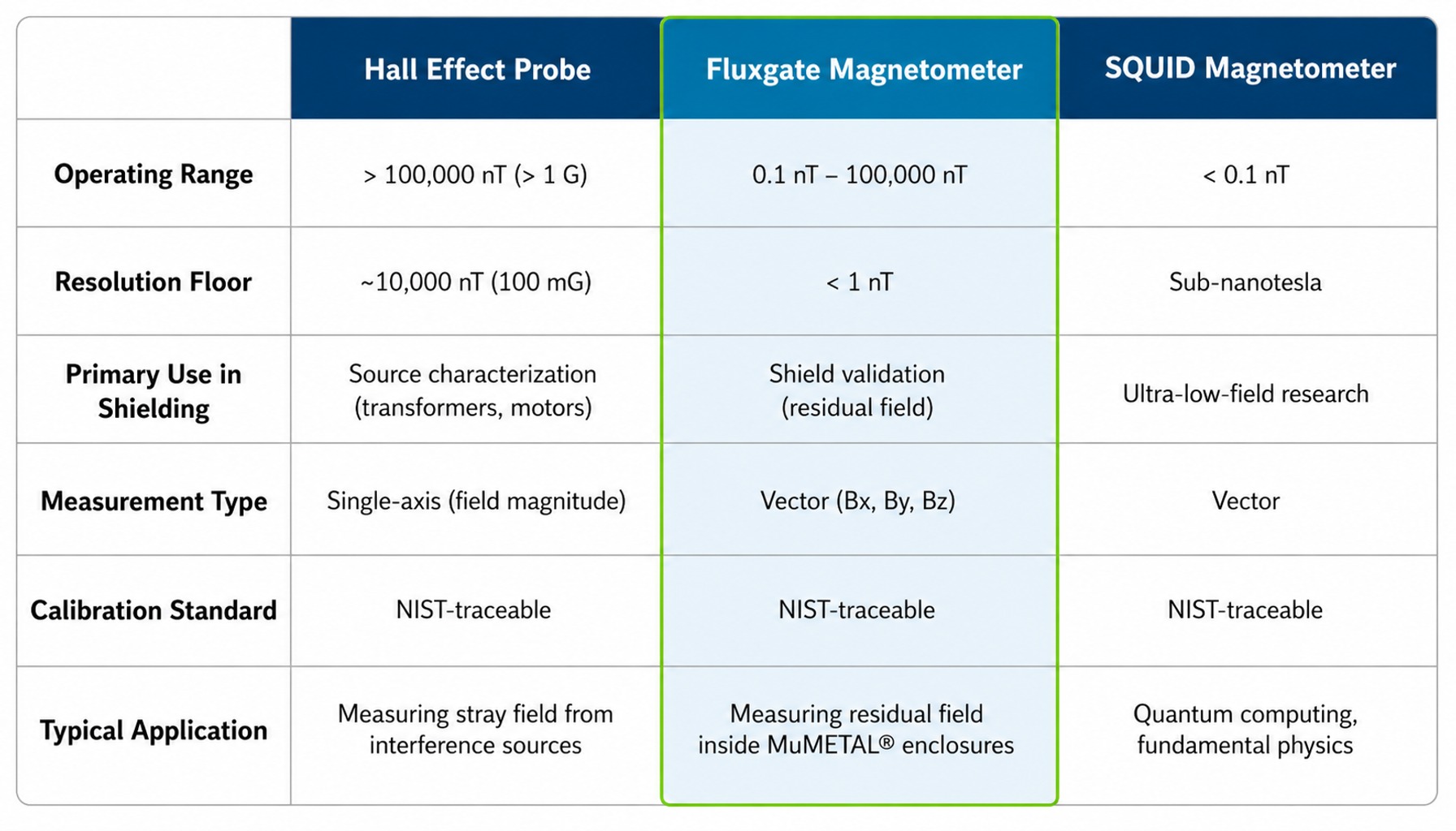
Instrument selection is the first critical decision point, and the most frequent mistake is using a Hall effect gaussmeter for a measurement that requires a fluxgate magnetometer or vice versa. The choice depends almost entirely on the expected field strength.
Field strength is not the only consideration, however; the instrument must also capture the frequency content and all three axes of the field. A situation that recurs in practice: a team building a superconducting quantum interference device (SQUID) magnetometer enclosure reports a shielding factor of 500 based on a single DC gaussmeter reading. When the same enclosure is later tested with a three-axis fluxgate magnetometer at 60 Hz, the measured attenuation drops to roughly 80. The DC-only, single-axis reading provides a completely misleading picture of performance against the actual AC interference.
As a general rule:
- Hall Effect Probes are appropriate for characterizing strong fields, typically above 1 mT (10 G). They are used to measure the source of interference, such as a transformer or motor.
- Fluxgate Magnetometers are the workhorse for validating shields, operating in the sub-microtesla range where most residual field targets lie.
- SQUID Magnetometers are specialized instruments for the most demanding applications, capable of sub-nanotesla measurements for quantum computing and fundamental physics research, but their cost and operational complexity place them outside the scope of most industrial validation tasks.
For any measurement intended to support qualification, ensure your instrument has a current, NIST-traceable calibration certificate.
Fluxgate Magnetometers for Sub-Microtesla Shielding Validation
For validating the performance of a high-permeability shield, the fluxgate magnetometer is the standard instrument. It is designed to operate with high resolution and stability in the 0.1 nT to 100,000 nT range.
A fluxgate operates by using a drive coil to periodically saturate a high-permeability core. The presence of an external DC or low-frequency AC magnetic field along the core's axis creates an asymmetry in the saturation, which produces a signal in a secondary pickup coil at the second harmonic of the drive frequency. The amplitude of this second-harmonic signal is directly proportional to the external field component.
Key characteristics of fluxgate sensors:
- Vector Measurement: A fluxgate measures the field component along a single axis. A three-axis measurement requires either a sensor head with three orthogonal cores or careful, sequential repositioning of a single-axis probe.
- Low Noise Floor: Performance is specified by noise spectral density, typically in nT/√Hz. A low noise floor is critical for resolving nanotesla-level residual fields. The 1/f noise corner frequency determines the instrument's stability for long-duration DC measurements.
- Industry Standards: The IEC 61786 standard provides detailed guidance on methods for measuring low-frequency magnetic and electric fields with respect to human exposure, and its principles are applicable to shielding validation.
Manufacturers such as Stefan Mayer Instruments and MEDA offer fluxgate magnetometers suitable for these applications.
Hall Effect Probes for High-Field and Material Characterization
Hall effect probes are essential for characterizing the magnetic environment before a shield is designed, when the task is to quantify the strong stray field produced by the interference source itself.
The operating principle relies on the Hall effect: when a current flows through a semiconductor (the Hall element), a magnetic field perpendicular to the current flow generates a voltage (the Hall voltage) across the element. This voltage is proportional to the field strength. Instruments like the gaussmeters from Lakeshore Cryotronics are widely used for this purpose.
However, a typical Hall probe has a resolution floor around 10,000 nT (100 mG). This is simply not sensitive enough to characterize residual fields inside a well-designed MuMETAL® enclosure, where targets are often below 100 nT. Using a Hall probe to measure a low residual field is like using a truck scale to weigh a letter; the instrument's resolution is coarser than the quantity being measured.
Establishing an Ambient Baseline Before Shielding Measurement
A shielding factor is a ratio: the ambient field strength divided by the residual field strength inside the shield. An inaccurate ambient measurement corrupts this ratio just as badly as an inaccurate internal measurement. It's a mistake we see often.
Consider this scenario: an engineer measures the ambient field at a planned shield location on a Saturday, when the building is quiet. They record a DC field of 48,000 nT. On Monday, they install the shield and measure a residual field of 120 nT, calculating a shielding factor of 400. What they miss is that during the weekday, the building's HVAC system, elevators, and nearby lab equipment generate a 60 Hz AC field of 1,500 nT that isn't present on the weekend. The true ambient environment is never characterized, and the calculated shielding factor is meaningless for the actual operating conditions.
A proper baseline characterization is not optional. The protocol is:
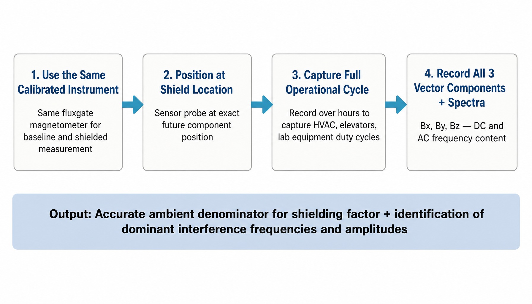
- Use the Same Instrument: Use the same calibrated fluxgate magnetometer for the baseline measurement that you will use for the shielded measurement.
- Measure at the Shield Location: Place the sensor probe at the exact location where the shielded component will reside.
- Capture the Full Operational Cycle: Record the magnetic field over a time window that is representative of the facility's full operational state. This could be minutes or hours, long enough to capture the duty cycles of elevators, HVAC systems, and other intermittent sources.
- Record All Components: Measure and record all three orthogonal B-field vector components (Bx, By, Bz) and their frequency spectra. This will reveal both the static (DC) field dominated by Earth's magnetism and the dynamic (AC) fields from electrical infrastructure.
This baseline measurement does two critical things: it provides the accurate "ambient field" denominator for your shielding factor calculation, and it identifies the dominant frequency and amplitude of the interference you need to shield against.
How to Measure Magnetic Field Strength Inside a Shielded Enclosure
Once you have a shield prototype on the bench and a calibrated fluxgate magnetometer, the quality of your data depends on your measurement protocol. Most errors in shielded measurements originate from three sources: probe standoff distance from the shield wall, sensor orientation, and the instrument's cross-axis sensitivity. A single reading at an uncontrolled position inside a shield is not a shielding factor measurement it is a number without context.
Probe Standoff Distance and Near-Wall Field Gradients
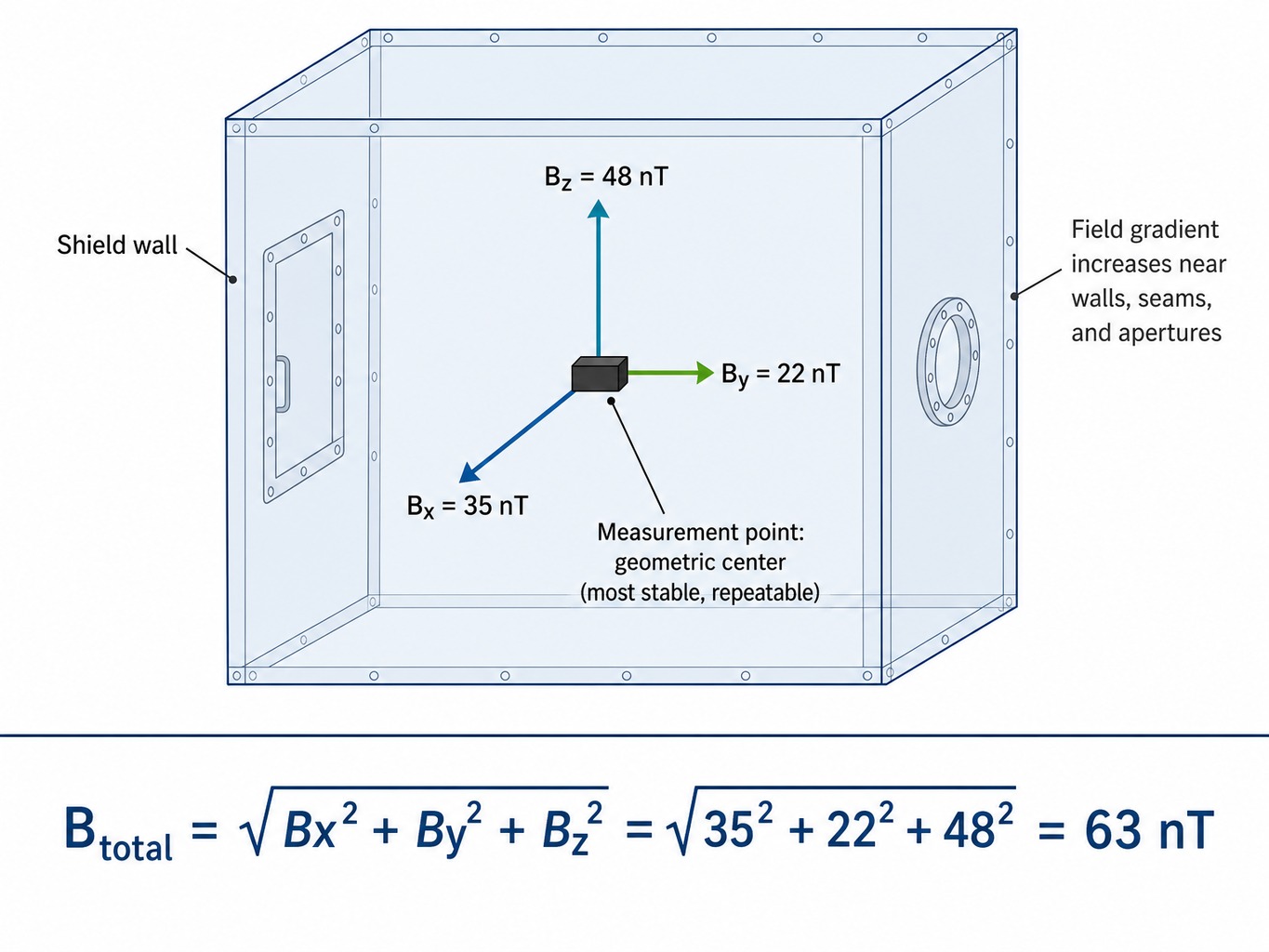
The magnetic field inside a high-permeability shield is not uniform. It is lowest at the geometric center and increases sharply near walls, seams, and any apertures. This is because the shield works by redirecting magnetic flux into the high-permeability material of the wall. Where an aperture is fitted with a shielding collar, confirm that the collar extends outward by a distance equal to or greater than the longest edge of the aperture or the hole diameter before you measure; a shorter collar leaves the opening as a leakage path and steepens the gradient around it. A rectangular sensor probe placed in this steep gradient region will produce a reading that is highly dependent on its exact position and orientation.
As a practical rule, all standard shielding factor measurements should be taken at the geometric center of the enclosure. This provides the most stable and repeatable measurement point, representing the best-case attenuation. If your specification requires field mapping at other coordinates, those points must be clearly defined and documented along with the standoff distance from the nearest wall.
If the enclosure is small, the physical size of the probe itself can become a factor. A sensor element that is large relative to the field gradient it sits in will average the field across its active area, potentially underreporting the peak field. Always note the probe's dimensions and its minimum standoff distance from any internal surface in your test report.
Three-Axis Measurement and Sensor Orientation Protocol
A single-axis magnetometer reading only captures one vector component of the residual field. Depending on how the probe is oriented relative to the dominant field direction, this single reading can dramatically understate or overstate the total field magnitude.
The correct protocol is to measure all three orthogonal B-field components (Bx, By, Bz) and calculate the total field magnitude as the vector sum:
B_total = √(Bx² + By² + Bz²)
Three-axis fluxgate sensors simplify this process by measuring all three components simultaneously. If using a single-axis sensor, you must perform three sequential measurements, carefully repositioning the probe at 90-degree angles and documenting the orientation for each reading.
Before starting, the sensor's offset should be nulled. This is best done by placing the probe inside a zero-gauss chamber to remove all external fields and adjusting the instrument output to zero. Also, be aware of cross-axis sensitivity. Even a three-axis sensor has finite rejection of off-axis fields, which can introduce small errors if one field component is much larger than the others.
Why a Single DC Reading Cannot Characterize Shield Performance Below 100 kHz
Most engineers default to a DC field measurement when validating a shield. That approach is incomplete, because DC attenuation and AC attenuation arise from different physical mechanisms. A shield that performs well at DC may offer significantly different performance at 60 Hz or 10 kHz.
The physics are distinct:
- DC Shielding relies on flux shunting. The high-permeability material provides a low-reluctance path that diverts the static magnetic field lines around the shielded volume. Performance is a function of the material's relative permeability and the shield's geometry.
- AC Shielding adds a second mechanism: eddy currents. The time-varying magnetic field induces circulating currents in the conductive shield wall. These currents generate their own magnetic field that opposes the incoming field. This effect depends on the wall thickness relative to the material's skin depth at the frequency of interest.
For high-permeability alloys like MuMETAL® (an 80Ni5Mo15Fe alloy conforming to ASTM A753 Alloy 4 / UNS N14080), the skin depth at 60 Hz is only a fraction of a millimeter. This means that even thin foil gauges of 0.152mm (.006"), 0.2mm (.008"), or 0.254mm (.010") provide a measurable eddy-current contribution at power frequencies. A standard 1.58mm (.062") sheet of MuMETAL® represents several skin depths.
If the dominant interference source for your application is a 60 Hz field from building power, a DC shielding factor does not predict how well the shield will attenuate the actual problem. Your measurement protocol must include spectral characterization of the residual field across the entire frequency range of concern, typically up to 100 kHz for these materials.
Measuring Before and After Hydrogen Annealing: Quantifying the Permeability Increase
The shielding performance of an enclosure made from an alloy like MuMETAL® or Co-NETIC® is almost entirely dependent on its final heat treatment. Fabrication stresses from bending, forming, welding, or punching can cause the relative permeability to plummet from a starting value of 10,000–25,000 down to as low as 100–1,000.
After a final, perfection-annealing cycle in a controlled dry hydrogen atmosphere, the permeability is restored and enhanced. As a result, permeability increases by a factor of 40 to 400, and shielding performance rises accordingly. Measuring the shield's performance both before and after this critical step is the only way to empirically verify that the annealing was successful and the shield meets its design intent.
The protocol involves a Helmholtz coil system, which generates a known, uniform magnetic field:
- Place the as-fabricated (unannealed) shield inside the Helmholtz coil.
- Apply a known field (e.g., 1 Gauss).
- Measure the residual field at the geometric center with a fluxgate magnetometer. Calculate the initial shielding factor.
- Perform the final dry hydrogen anneal on the shield.
- Place the annealed shield back in the identical test setup.
- Apply the same known field and repeat the residual field measurement. Calculate the final shielding factor.
If the measured improvement falls well short of the expected 40 to 400 times permeability recovery, it indicates a problem either the annealing cycle was incomplete, or the part was mechanically stressed after annealing. Even minor post-anneal work like drilling a hole or rough handling can locally degrade permeability, compromising the entire shield. This is why final annealing must be performed after all mechanical work, including welding, is complete.
Correlating COMSOL Simulation Predictions with Physical Magnetometer Readings
Finite element analysis software like COMSOL Multiphysics® predicts field attenuation in a proposed shield design. However, a simulation is only as reliable as its inputs. The B-H curve used in a COMSOL® model must correspond to the actual thermomagnetic history of the material in the fabricated part, not a textbook curve for the alloy family.
The correct engineering workflow is complementary: simulate to design, measure to validate.
- Build the simulation model using realistic material properties (permeability curves from measured data, like that from ASTM A773 tests).
- Fabricate a prototype based on the model.
- Measure the prototype's performance using a disciplined protocol under the same ambient conditions modeled in the simulation.
- Compare the measured residual field to the simulation's prediction.
Discrepancies are diagnostic. They typically trace to one of three sources: the permeability value in the model was too optimistic, the model didn't account for flux leakage through real-world seams or apertures, or the ambient field conditions in the lab didn't match the boundary conditions in the simulation. By systematically investigating these gaps, teams can refine their models and converge on a validated design.
From Measurement Data to Validated Shield
To summarize: valid magnetic field measurement requires the right instrument, a disciplined baseline, frequency-aware protocols, and pre- and post-annealing comparison. Measurement is only one part of that chain; the shield must also be fabricated, annealed in a high-temperature dry hydrogen furnace, and then tested in a controlled laboratory.
At Magnetic Shield Corporation, that chain begins with proprietary alloys like MuMETAL®, Co-NETIC®, NETIC®, and CRYO-NETIC®, continues through custom fabrication including precision welding, and ends with final hydrogen annealing.
We validate performance in our quality laboratory. Using Helmholtz coil systems, calibrated magnetic-field sensors, and a controlled environment, we test finished shields to standards like ASTM A773 and ASTM A698. This process connects the design prediction to a documented, measured result, with COMSOL® simulation and an online shielding calculator supporting the design side.
A reliable magnetic shield is an engineered system, and the process of verifying its performance must be equally engineered.
As applications in quantum computing and aerospace push residual field requirements into the single-nanotesla range, this measurement discipline is what confirms that a shield's predicted attenuation holds under real operating conditions.
Engineers validating shield performance can request application support to Magnetic Shield Corporation.
Frequently Asked Questions
What measurement resolution in nanotesla is needed for quantum computing magnetic shielding validation?
Quantum computing and SQUID-based systems often require residual fields below 10 nT, and sometimes below 1 nT. This demands a fluxgate magnetometer with a noise floor at or below 0.1 nT/√Hz, or a SQUID for the most sensitive work. Your instrument's resolution should be at least 10 times better than your target residual field.
How often should fluxgate magnetometer probes be recalibrated for reliable shielding validation?
Most manufacturers recommend annual recalibration traceable to NIST standards. However, any probe subjected to mechanical shock, extreme temperatures, or strong field exposure should be checked immediately. For qualification-critical projects, it is good practice to verify calibration against a known reference source, like a Helmholtz coil, before each major test campaign.
What is the correct procedure for measuring permeability per ASTM A773?
ASTM A773 specifies a ballistic test method using a toroidal ring specimen of the material, which is wound with primary (magnetizing) and secondary (sensing) coils. A known magnetizing force (H) is applied via the primary coil, and the resulting change in magnetic flux (B) is measured by integrating the voltage from the secondary coil, allowing for direct calculation of the material's B-H curve and permeability.
What magnetic field measurement equipment is required for aerospace EMI compliance testing?
Aerospace compliance testing, such as for standards like DOD-STD-1399-070 Part 1, typically requires a calibrated three-axis fluxgate magnetometer with sub-microtesla resolution and documentation traceable to NIST standards. A Helmholtz coil system is often used to generate reference fields for susceptibility testing. Specific requirements vary by program and prime contractor.
Can a gradiometer configuration improve magnetic field measurement accuracy inside a shield?
A gradiometer, which uses two spaced sensors to measure the field gradient, is effective at rejecting common-mode noise from distant sources. Inside a shield, it can help distinguish a true residual field from sensor drift or uniform noise leaking through. However, it measures the gradient (dB/dx), not the absolute field, so it supplements rather than replaces a single-sensor magnetometer for standard shielding factor validation.
How does CRYO-NETIC® differ from MuMETAL® for magnetic field measurement at cryogenic temperatures?
CRYO-NETIC® is a proprietary nickel-iron alloy specifically engineered to maintain high magnetic permeability at cryogenic temperatures, down to near absolute zero (4 K). The permeability of standard MuMETAL® decreases significantly at these low temperatures. For shielding validation in cryogenic environments, the measurement must be performed at the actual operating temperature using a shield made from a material like CRYO-NETIC®.